
When we say something is complicated, what does that really mean? In grad school, I had a final that had just two problems. The first problem was, from basic principles, derive the full (no simplifications) Navier-Stokes equations. The second problem was to derive the full vorticity equations and identify what each term means. In high school, I had taken the Armed Services Vocational Aptitude Battery exam. The math portion had over 50 problems, but they were all simple arithmetic. So which was more complicated? The 50+ problems or the mere two?
I have heard over the years about how complicated dispersion modeling is. To perform dispersion modeling, you have to consider many moving parts. There are multiple data sets to consider like surface weather and upper-air observations, terrain elevations, land cover, and ambient monitoring. There are multiple computer programs to process the data sets like AERMET, AERMAP, AERSUFACE, AERMINUTE, and BPIPPRM to ready the data for AERMOD. There are a lot of details to attend to, but, to complete honest, dispersion modeling is really not that complicated.
Like the Armed Service Battery exam, there are dozens of elements to consider, but the vast majority are very simple, straightforward, and even tedious. There are areas where the true discretion and professional judgement come into play, but 90% of the effort is on tasks that anyone could do given proper instructions to follow.
What is “Discretion and Judgement”?
In putting together a dispersion modeling analysis, a bizillion selections need to be made. However, how many of those selections required any thought? If the selection is based on following instructions, then no thought at all is required. The difference between a technician and a professional is the technician follows a list of instructions. After a while, the instructions are just rote memory. If a selection involves comparisons or analysis, then that requires discretion (criteria for a decision) and judgement (the process of making the decision), that requires some thinking.
The Process and Time Line
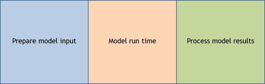
Below is a simple graphic showing the dispersion modeling process at a very high level. Basically, three parts: prepare the model input, run the model, and process the model results.
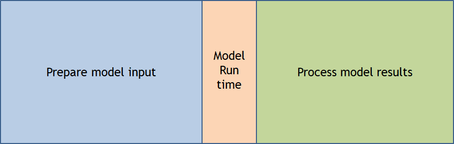
Back in the good old days (early 1990’s) when desktop computers were becoming a thing, model run time was a significant chunk of the time required to perform a dispersion modeling analysis.
Over time, technology got better, computer processors got faster, so model run time had been reduced in a big way. However, at the same time, more sophisticated models were developed requiring more data input, so the input preparation time increased. Also, as air quality standards became more stringent, it became less likely that a project was going to have an insignificant impact. As a result, more modeling analysis was going to be necessary to demonstrate compliance with air standards. The outcome was more modeling and more modeling results to be processed. The adjusted timeline is below.
Any gains made by faster CPUs was eaten up on the front end with more data requirements and the back end with more analysis and more results to process.
For the most part, performing a dispersion modeling analysis takes about the same amount of time and effort as it did 30 years ago. The reason why a dispersion modeling analysis takes no longer than it did 30 years ago is the process is performed, for the most part, in the same way and with the same tools as it was 30 years ago.
Improving the Process Time Line
To improve the process time (and effort), the process has to be improved. Below is a simplified list of the steps in the process:
- Define the site property line or fence line
- Generate receptor grid
- Select terrain data files
- Run AERMAP
- Select NWS surface and upper stations
- Download NWS data
- Download land cover data
- Run AERSURFACE, AERMINUTE, and AERMET
- Identify any nearby Class I areas, nonattainment areas, and affected states
- Identify which air contaminants to evaluate
- Determine air contaminant background concentrations
- Identify nearby monitors
- Download regional emissions data
- Download emissions data for nearby sites
- Download land cover data
- Determine air contaminant background concentrations
- Identify emission sources included in evaluation
- Obtain from applicant:
- source IDs
- Source locations
- Source exhaust parameters
- Source operating schedule
- Source emission rates
- Building/Structure locations and height
- Run AERMAP for source and building elevations
- Run BPIPPRM
- Obtain from applicant:
- Determine source characterizations
- Document selection of source type
- Define modeling scenarios
- Define source groups
- Select output options
- Execute model
- Compile model results
- Generate analysis report
For the most part, these are all the steps involved. Some may not be needed in some case, but this is a comprehensive list of task.
Take a look at the list and ask yourself how much actual thought goes into making a selection or completing the task. Selecting which file to download, provided you know where to find the data, does not require any thought. Data entry does not require any brainpower.
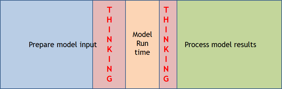
Of the 30+ steps listed above, maybe a handful truly requires any discretion and professional judgement. The graphic below depicts the approximate amount of thinking time goes into a typical dispersion modeling analysis.
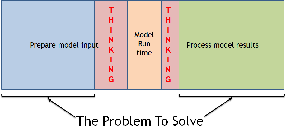
If you want to shorten the time and effort necessary for a dispersion modeling analysis, your options are limited. There isn’t much you can do to shrink model run time. You really don’t want to reduce the amount of thinking time as there is a shortage of that already. The place to attack the problem is at all the non-thinking, non-discretionary, and non-judgement tasks.
What Makes NaviKnow Different
If you are solving the wrong problem, you are not going to find a workable solution to the real problem. In this article, we have laid out our analysis of the problem and have shown where the real problems lie.
In the next few articles, we will be providing access to tools that make a real difference reducing the time, effort, and cost of performing dispersion modeling analyses.
The solutions we pose is not something we can create and construct in a vacuum. We don’t believe in the “build it and they will come” business model. We will require input into the process and buy into the concepts from the regulators and the regulated. If you want to be a part of the solution, contact us to start the dialog.
If you found this article informative, there is more helpful and actionable information for you. Go to http://learn.naviknow.com to see a list of past webinar mini-courses. Every Wednesday (Webinar Wednesday), NaviKnow is offering FREE webinar mini-courses on topics related to air quality dispersion modeling and air quality permitting. We also have articles about air quality issues at http://naviknow.com/news. If you want to be on our email list, drop me a line at [email protected].
One of the goals of NaviKnow is to create an air quality professional community to share ideas and helpful hints like those covered in this article. So if you found this article helpful, please share with a colleague.