
If you are into woodworking, then you know what a jig is. It takes a bit of time to put one together. Once you have it and use it, it’s like magic. You will ask yourself, “why didn’t I do this sooner?”
The NaviKnow Air GeoDataBase is like a collection of jigs for most of your air quality data analysis needs. For the whole month of February, we are going to walk you through how use the Air GDB to save you time and effort. Each week we will demonstrate it use for a specific topic.
Background Concentrations for Dispersion Modeling
What does a geodatabase have to do with coming up with a representative pollutant background concentration? Well, to be honest, it has everything to do with it. Though it does seems like magic, you can’t just pull a value out a hat and tell a regulator, “here it is.” There has to be a process and, more importantly, documentation on how the value was arrived at.
Using the Air GDB to determine a representative background pollutant concentration provides for a process that is:
- realistic,
- reproducible,
- systematic, and
- objective.
With these qualities, the process generates the documentation as you step through it.
Background on Background
The US code of federal regulations (CFR) states the following:
40 CFR 51.166(m)(1) – Preapplication Analysis
(i) The plan shall provide that any application for a permit under regulations approved pursuant to this section shall contain an analysis of ambient air quality in the area that the major stationary source or major modification would affect for each of the following pollutants:
(a) For the source, each pollutant that it would have the potential to emit in a significant amount; (new major source)
(b) For the modification, each pollutant for which it would result in a significant net emissions increase. (major modification)
40 CFR 51 Appendix W 8.3.2
If several monitors are available, preference should be given to the monitor with characteristics that are most similar to the project area. If there are no monitors located in the vicinity of the new or modifying source, a “regional site” may be used to determine background concentrations. A regional site is one that is located away from the area of interest but is impacted by similar or adequately representative sources.
Summarizing the citations from the CFR, if your project triggers a NAAQS demonstration, you are required to estimate the air quality where the project site is located. If you choose to use ambient air monitoring data to make that estimate, the areas surrounding the project site and the selected monitor should be similar.
Two clues as to how an analysis can be conducted are the terms “characteristics” and “sources”. These terms can be translated as “land use” and “emissions”. These clues provide the basis for the process described in this article. In stepping through the process, we will compare, between the project site location and potential monitor locations, the similarity of:
- Regional emissions,
- Nearby emissions, and
- Nearby Land Use.
Using the Air GDB to Determine Background Concentrations
To make the comparison of emissions and land use between two locations using the Air GDB, the datasets we will use are:
- National Emissions Inventory (NEI) County-Wide emissions,
- NEI Major source emissions, and
- Monitor design values.
First, launch ArcMap. To fill in your blank map, click on the Add Data icon ![]()
Locate where you have the Air GDB, then expand it to see all the datasets available. There are four datasets to add for this example:
- COUNTIES_USA,
- SITES_NEI,
- MONITORS, and
- PROPERTY_LINES.
The PROPERTY_LINES dataset was obtained from the Texas Commission on Environmental Quality (TCEQ). It contains property boundaries of industrial sites in Texas. This dataset is being used because an application site (industrial site seeking a permit) is needed to start the whole process. You can use any dataset you like that has an application site specific to you dispersion modeling project.
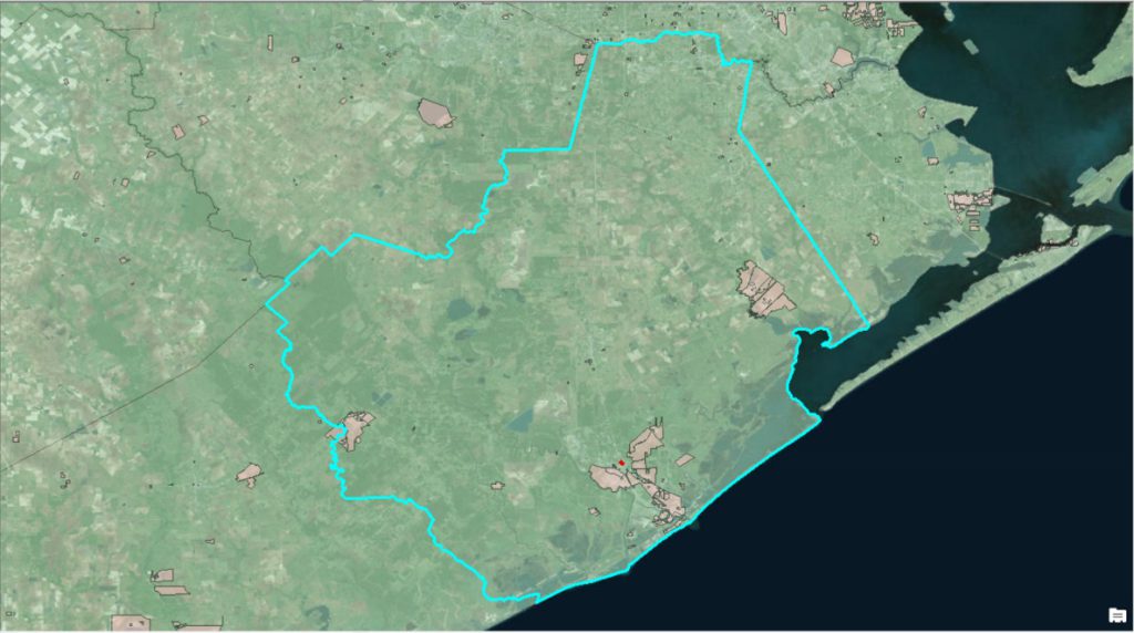
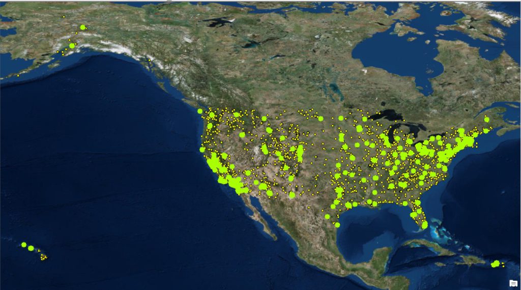
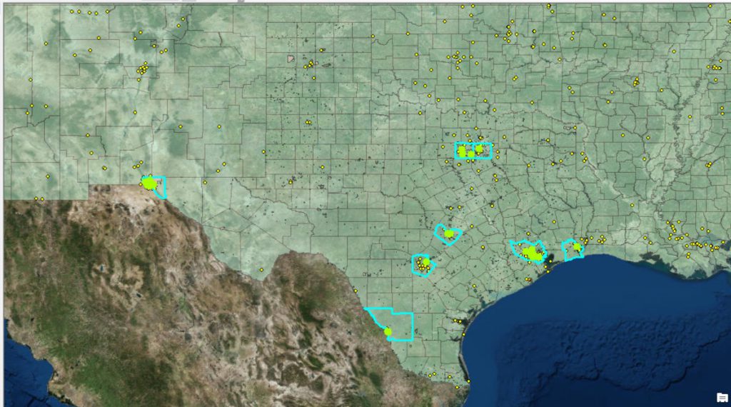
Your map display should look something like this:
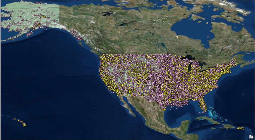
The ambient air monitors are depicted in yellow, the industrial sites (from the NEI and TCEQ) are in rose, and the counties are in light green.
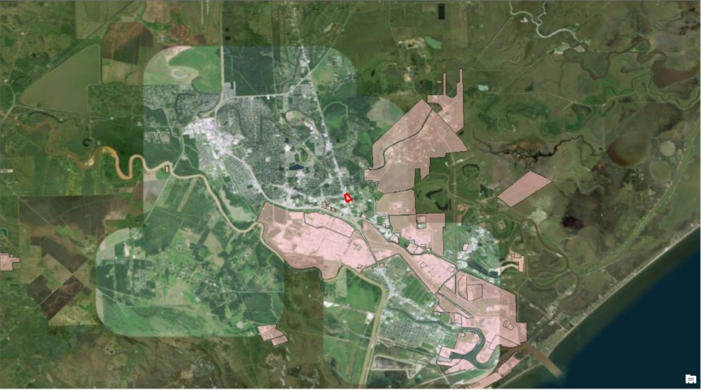
Next, select the location of the application project site from PROPERTY_LINES by using the Select Features icon ![]()
For this example, we have chosen a site in southeastern Texas (in red). Our map display looks like this:
County-Wide Emissions Analysis
Project Site County
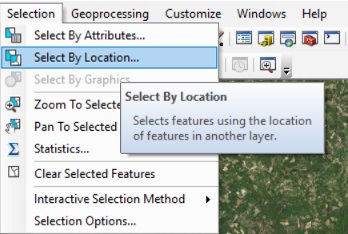
Once we have selected a project site, the first step is to look up the emissions for the county where the site is located. To access the county-wide emissions, we perform a spatial query between the two datasets; PROPERTY_LINES and COUNTIES_USA. To do so, click on the Selection menu item and then click on Select By Location…
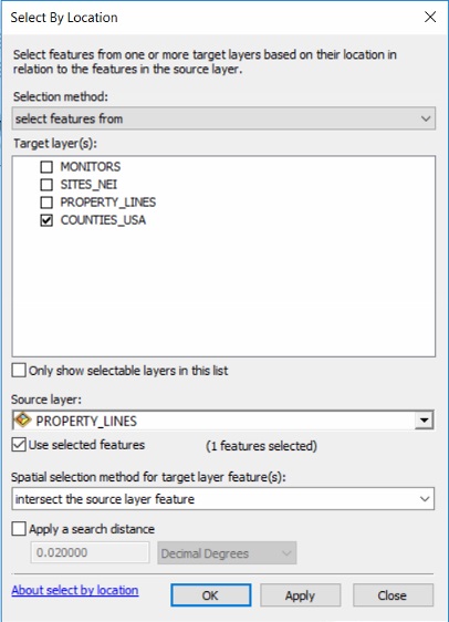
What we want to do is select features from COUNTIES_USA that intersect with the location of the selected feature from PROPERTY_LINES. The Select By Location dialog form would look like this:
Click the Apply or OK button the execute the query. Zooming out in the map display to show all (one) the counties meeting the query criteria (in bright blue), our display looks like this:
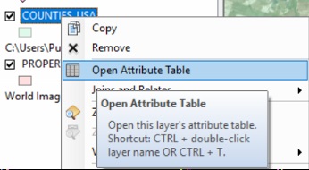
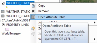
After we have selected the county for our project site, we will need to access the data associated with that county. To do so, right-click on the COUNTIES_USA dataset, then select Open Attribute Table.
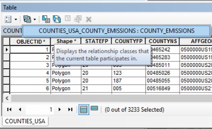
We will see the selected record in bright blue. In the COUNTIES_USA attributes table, only identifying information is contained in this table. The county-wide emissions data is located in a related table. To access the related table with emissions data, click on the related tables icon ![]()
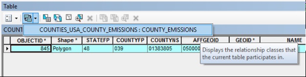
And then select COUNTY_EMISSIONS. This will open the data table containing the related records for the county-wide emissions. Your display should look similar to this:
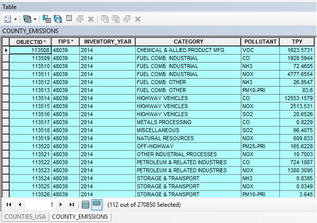
At this point, we do not need all 112 selected records. For our initial filter of the data, we are only interested in the total emissions for the county, not the individual source categories. To apply this filter, click on the Select By Attributes button. ![]()
The Select by Attributes dialog box opens, listing the data fields to filter (query) on. We want to select those records, selected from the current selection, that have the category TOTAL. The dialog box should look like this:
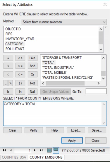
It is important to note, the Method: text box is set to Select from current selection. If you do not set this properly and leave it on the default setting Create a new selection, the query will be on all 270,850 records and not on the 112 needed.
Click the Apply button to execute the query. The result will look like this:
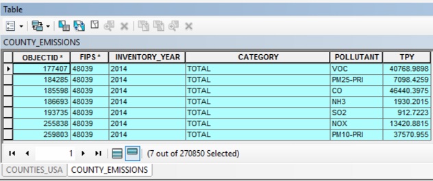
This table lists the total emissions of criteria pollutants for the county of our project application site. Now that we know the emissions for this county, next we will identify which counties have comparable emissions AND contain an ambient air monitor. To make this comparison, we will need to do so pollutant by pollutant. For this example we will consider only carbon monoxide (CO). For the other criteria pollutants, the steps to follow are identical.
For our example, the county-wide total emissions are 46,440 TPY. Next we will select from the COUNTIES_USA dataset those counties that contain at least one CO monitor.
Counties with a Carbon Monoxide Monitor
One of the powers of using GIS data (spatial data) is the data allow the comparison of completely different datasets that only have one thing in common: location. First we will identify all the CO monitors, then identify counties that are similar, based on total CO emissions, and finally identify the overlap between the two datasets.
Where are the CO Monitors?
Now, we will query the MONITORS dataset by right-clicking on the MONITORS dataset, then select Open Attribute Table.
The attribute table for MONITORS only contains minimal identifying information. To access the data listing which pollutants a monitor samples, click on the related tables icon, then select MONITOR_POLLUTANTS.
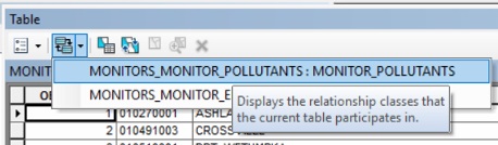
We do not need every record in MONITOR_POLLUTANTS, only those associated with CO. To filter to only the CO related records, we will need to query this data table. To do so, click on the Select By Attributes button.
The Select by Attributes dialog box opens, listing the data fields to filter query on. We want to select only those records where the POLLUTANT value is CO. The Select by Attributes dialog should look like this:
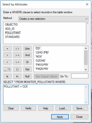
Click the Apply button to execute the query.
All the records that met our criteria are selected, but we want the location of the monitors that meet our criteria. To do so, click on the related tables icon, then select MONITORS.
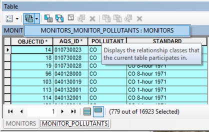
The result should like something like this:
Which Counties Are Similar to Project County?
To select which counties have similar total emissions to our project application site, we will need to query the COUNTIES_USA dataset and the related table COUNTY_EMISSIONS. To do so, right-click on the COUNTIES_USA dataset, then select Open Attribute Table.
To access the COUNTIES_EMISSIONS table, click on the related tables icon, then select COUNTY_EMISSIONS.
To select the counites that are similar based on total CO emissions, we will want to query the COUNTY_EMISSIONS table for records where the CO emissions are at least as high as our project site county. To build this query, click on the Select By Attributes button.
The Select by Attributes dialog box open. We want to select only those records where the POLLUTANT value is CO, the total CO emissions are greater than 46,400, and, since Texas has many monitors that are nearby, we are only considering monitors in Texas. The Select by Attributes dialog should look like this:
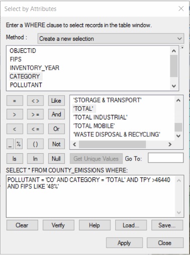
Click the Apply button to execute the query.
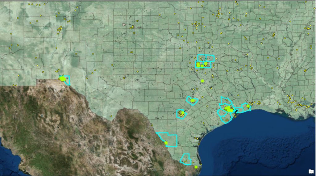
To show where the counties are located, click on the related tables icon, then select COUNTIES_USA. The display of selected counties (bright blue) and selected monitors (bright green) should look like this:
Making the Comparison
Now that we have narrowed the list of counties and monitors to just a few, we will need to narrow a little more by looking at the overlap of the two data sets. To do so, click on the Selection menu item and then click on Select By Location…
What we want to do is select features from the selected COUNTIES_USA that intersect with the location of the selected features from MONITORS. The Select By Location dialog form would look like this:
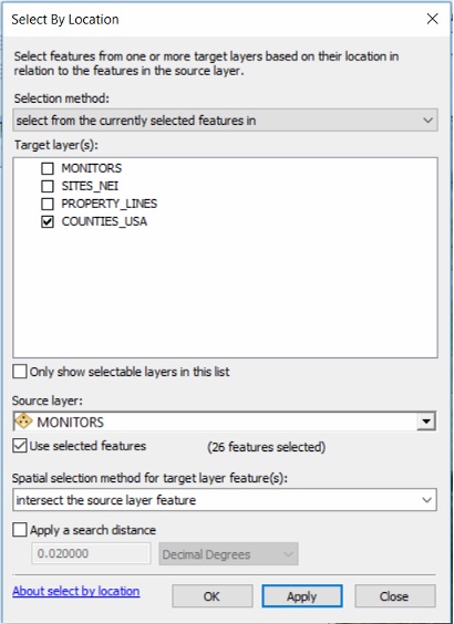
Note in the Selection method list box we chose select from the currently selected features in and not from all of the monitors in the dataset. The results are the overlapping counties.
Flipping around the Target and Source layers to get the overlapping monitors, the dialog box looks like this:
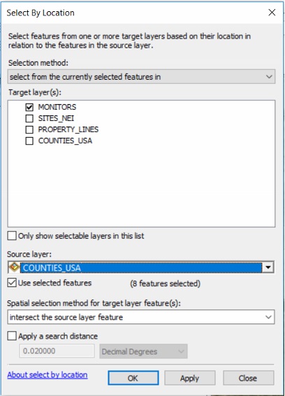
The display should look like this:
Though we haven’t gotten to a final result, the analysis thus far has narrowed our search to about a dozen potential monitors that could be considered representative. Performing the nearby emissions analysis will narrow down the list some more.
Nearby Emissions Analysis
The nearby emissions analysis looks at annual emissions for industrial sites within 10 kilometers (km) of our project site.
Project Site Nearby Emissions
To determine the nearby emissions for the project site, we perform a spatial query between the two datasets; PROPERTY_LINES and SITES_NEI. To do so, click on the Selection menu item and then click on Select By Location…
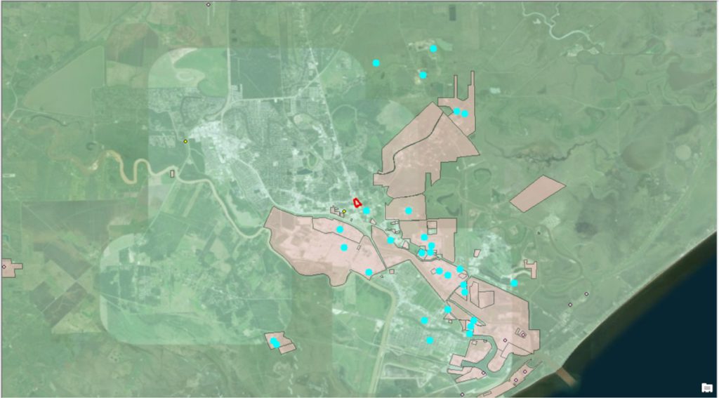
What we want to do is select features from SITES_NEI that are within 10 km of the location of the selected feature from PROPERTY_LINES (our project site). The Select By Location dialog form would look like this:
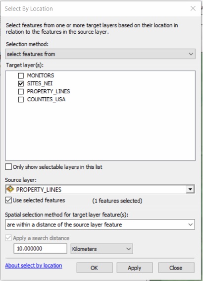
The spatial query results are displayed below. The selected sites are bright blue.
This display shows the locations of nearby sites, but we need to access the annual emissions of these site. To do so, right-click on the SITES_NEI dataset, then select Open Attribute Table.
To access the emissions table, click on the related tables icon, then select SITE_NEI_EMISSIONS.
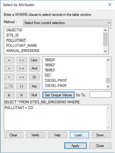
To select the nearby site CO emissions, we will want to query the SITE_NEI_EMISSIONS table for records with CO emissions. To build this query, click on the Select By Attributes button.
The Select by Attributes dialog should look like this:
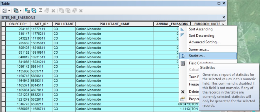
Click on the Apply button to execute the query. The result shows all the individual emission rates, however, we want the total emissions from all of these sites. To do this, right-click on the ANNUAL_EMISSIONS field, then select Statistics… See the display below.
The Selection Statistics dialog box will open, displaying several aggregate values based on the selected records. One of those items is Sum.
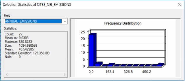
For our project application site, the total CO emissions from nearby sources is 1,095 TPY.
Monitor Nearby Emissions
To determine the nearby emissions for potentially representative monitors, we can use the narrowed list of monitors we have from the county-wide emissions analysis. We will query the MONITORS dataset by right-clicking on the MONITORS dataset, then select Open Attribute Table.
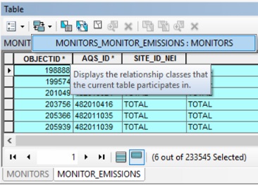
The attribute table for MONITORS only contains minimal identifying information. To access the data listing which pollutants a monitor samples, click on the related tables icon, then select MONITOR_EMISSIONS.
The MONITOR_EMISSIONS table lists the emissions of sites from the NEI within 10 km of each monitor and the total emissions of all those sites listed individually.
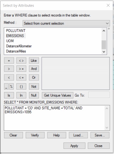
The next step is to query the MONITOR_EMISSIONS table for the total emissions of CO greater than 1,095 TPY. To build this query, click on the Select By Attributes button.
The Select by Attributes dialog should look like this:
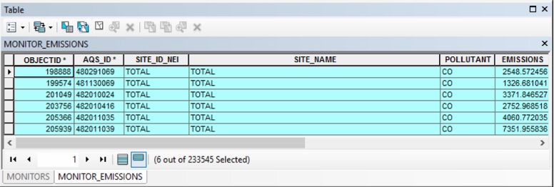
Click on the Apply button to execute the query. The result has narrowed the list of potential representative monitors further. The results are shown below.
To see where these monitors are, click on the related tables icon, then select MONITORS.
Making the Selection
Through our analysis, we have evaluated and compared the county-wide emissions of our project site to all other counties with a CO monitor, and narrowed the list of similar counties to three. We have also evaluated and compared the emissions of industrial source within 10 km of our project site and CO monitors, and narrowed the list of representative monitors to six. Without further analysis, all six monitors could be considered representative of the area surrounding our project site. The next step is to select a representative monitor and determine a representative background concentration for CO.
In our previous step of the procedure, we left with the attribute table of MONITORS showing the six monitors that met our similarity procedure. Next we want to see what the design values are for each of these monitors. To access the monitor design values, click on the related tables icon, then select MONITOR_DESIGN_VALUES.
The remaining values to choose from look like this:
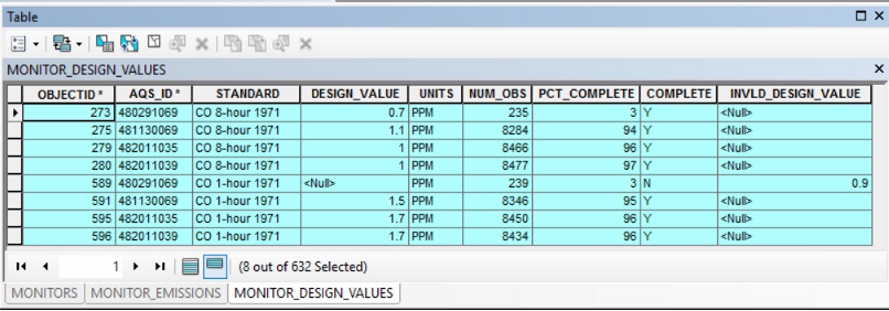
At this point, having gone through this analysis, any of these values could be considered representative.
Summary
The procedure described in this article seems like a lot of steps to take and can take a few minutes to go through. We agree. However, if you do not follow a process that is realistic, reproducible, systematic, and objective, you may end up spending days or weeks trying to explain and document how you came up with a background concentration value.
If you found this article informative, there is more helpful and actionable information for you. Go to http://learn.naviknow.com to see a list of past webinar mini-courses. Every Wednesday (Webinar Wednesday), NaviKnow is offering FREE webinar mini-courses on topics related to air quality dispersion modeling and air quality permitting. If you want to be on our email list, drop me a line at [email protected].
One of the goals of NaviKnow is to create an air quality professional community to share ideas and helpful hints like those covered in this article. So if you found this article helpful, please share with a colleague.
If you are interested in learning more about the NaviKnow Air GDB, go to http://www.naviknow.com/geodatabase/. You are welcomed to give it a test drive by going to http://www.naviknow.com/geodatabase-trial/ for a 30-day trial.
Resources